Working with the posterior¶
A topic-organized walk through the posterior’s analysis surface — fitting, inspecting, allocating, deciding, verifying. The narrative “day in the life” of a data scientist running a real adaptive experiment lives in first adaptive experiment; this doc is the reference companion you reach for when you know what capability you need and want to see it isolated.
Each section covers one capability, shows the canonical method call, and explains how the output composes with the other methods. The joint posterior is the root primitive everything derives from — see result objects for the type hierarchy.
Setup¶
import os
os.environ.setdefault("JAX_PLATFORMS", "cpu")  # delete this line to run on your GPU

import pytyche as pt
To confirm your JAX platform, GPU availability, and library versions,
run pt.check_setup().
The runnable examples use pytyche’s clustered_realistic generator
so the tutorial is self-contained:
from pytyche.generators.core import generate_v2_core

config, _meta = pt.generators.clustered_realistic(
    "revenue_per_visitor", 1.0, K=3, n_visitors=2_000, seed=42
)

bundle = generate_v2_core(config)
observed, truth = bundle
pt.generators.<name>(...) is the attribute-access sugar for
pt.TEMPLATES["<name>"](...) — both resolve to the same registered
template function. The first two positional arguments are metric_id
(e.g. "revenue_per_visitor") and effect_scale (the planted signal
amplitude). K is the treatment count (control + K−1 active
treatments). The template returns a (V2GeneratorConfig, dict) tuple;
generate_v2_core(config) returns a CalibrationBundle — a
NamedTuple that unpacks to (observed, truth).
truth carries the ground truth the generator planted; the
truth comparison section uses it. Every other
section reads identically to what you’d write against real data.
§1 — Fitting and dispatch¶
pt.fit(observed) is the canonical entry point. It inspects the
data shape and dispatches to the right BCF flavor:
continuous outcome →
fit_continuous_bcfbinary outcome →
fit_binary_bcfzero-inflated outcome (hurdle) →
fit_hurdle_bcf
For the dataset above (zero-inflated revenue, three treatments) it dispatches to the joint multi-arm hurdle BCF.
Runtime
Expect this fit to take a few minutes on CPU, or about a minute on a GPU. The same code scales to hundreds of thousands of visitors on GPU — see your first hurdle BCF fit for sizing guidance.
posterior = pt.fit(
    observed,
    num_chains=2,
    num_mcmc=200,
    num_burnin=200,
    seed=42,
)
/builds/tradcliffe2/tyche/src/pytyche/bcf/dispatch.py:207: NoCudaWarning: No CUDA device detected — this fit runs on CPU, which is orders of magnitude slower at production scale. Install the GPU extra: uv add 'pytyche[gpu]' (or pip install 'pytyche[gpu]'). Set PYTYCHE_SUPPRESS_GPU_WARNING=1 to silence this warning.
  return selected(
If you want explicit control over the fit function (skipping the
auto-dispatch), call pt.fit_hurdle_bcf(observed, ...) directly.
The returned posterior is identical bit-for-bit when seeds and kwargs
match — pt.fit is a thin dispatcher, not a separate fit path.
The default pooling kwarg for hurdle outcomes is "joint" — the
canonical shared-tree fit that borrows strength across the conversion
and severity channels. Pass pooling="independent" (binary arm only)
for the two-stage baseline.
The posterior stashes observed on itself (posterior.observed), so
downstream methods don’t need it passed again. The default copy
semantics is view — posterior.observed is observed — which is what
you want for in-process flows. Pass observed_copy="deep" on pt.fit
if you need the posterior to retain an independent copy (serialization
across processes, mutation guarantees).
§2 — Inspection¶
posterior.analyze() produces the canonical analysis output — global
per-treatment contrasts plus a fitted policy-tree segmentation. This is
the single call that answers “what does the data say about this
experiment?”
The fit sees every feature column in the observed frame. For this
dataset that is five e-commerce features (session_recency,
browse_depth, device_type, is_returning, channel) plus five
noise columns (z0–z4) the generator added. Which columns carry
signal is truth-side knowledge the analysis path never receives —
the policy tree has to discover it from the CATEs alone, with the
no-signal columns competing for every split:
analysis = posterior.analyze()
analysis
| comparison | lift (80% CI) | P(lift > 0) |
|---|---|---|
| treatment_1 vs control | +11.2155 [+8.0849, +14.4382] | 1.00 |
| treatment_2 vs control | -2.6405 [-4.1202, -1.3419] | 0.01 |
| segment | share | GATE (80% CI) | stability | leader |
|---|---|---|---|---|
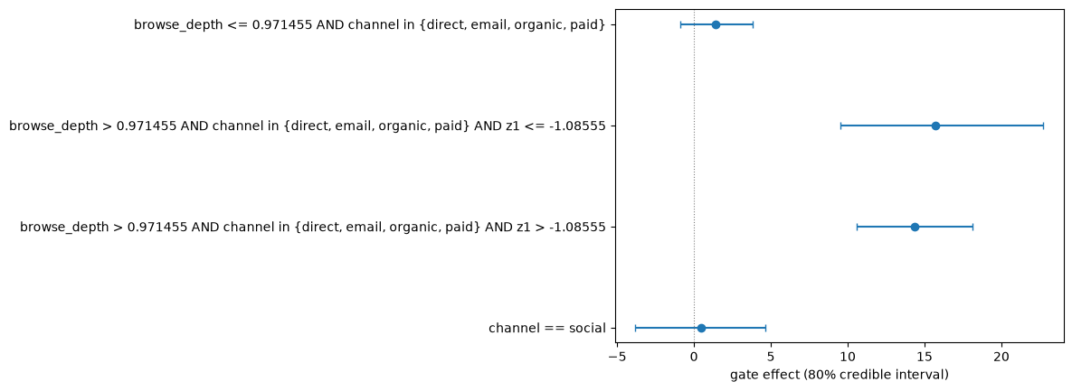
| browse_depth <= 0.971455 AND channel in {direct, email, organic, paid} | 11% | +1.4318 [-0.8810, +3.8104] | 1.00 | treatment_1 P=0.80 |
| browse_depth > 0.971455 AND channel in {direct, email, organic, paid} AND z1 <= -1.08555 | 10% | +15.6959 [+9.5160, +22.7293] | 0.46 | treatment_1 P=1.00 |
| browse_depth > 0.971455 AND channel in {direct, email, organic, paid} AND z1 > -1.08555 | 66% | +14.3664 [+10.5937, +18.1141] | 1.00 | treatment_1 P=1.00 |
| channel == social | 14% | +0.4482 [-3.8081, +4.6292] | 1.00 | treatment_1 P=0.55 |
recommendation: SHIP — treatment_1
If you have a segment hypothesis of your own (say, “mobile visitors
respond differently”), you don’t need analyze for it — declare the
segment with the rule algebra and ask the per-segment primitives
directly: posterior.recommendation_summary(treatment, segment=...)
gives the declared segment’s decision-theoretic snapshot, and
posterior.thompson_allocation(segments=[...]) its allocation. A
higher-level convenience for declaring segment hypotheses up front is
planned but not yet available; the compositional path above is the
supported route today.
Global contrasts¶
for comparison in analysis.comparisons:
    print(comparison)
Comparison — treatment_1 vs control
  lift: +11.2155   80% CI [+8.0849, +14.4382]   P(lift > 0) = 1.00
  decomposition — conversion: +0.0712 [+0.0500, +0.0907]   severity: +34.1756 [+13.2831, +55.3771]
Comparison — treatment_2 vs control
  lift: -2.6405   80% CI [-4.1202, -1.3419]   P(lift > 0) = 0.01
  decomposition — conversion: -0.0256 [-0.0412, -0.0110]   severity: -24.8586 [-46.4949, -2.0628]
P(lift > 0) is the posterior probability that the treatment beats
control at the population level. The lift point estimate and credible
interval are in outcome units (revenue per visitor, for this dataset).
The 80% credible interval is the contracts.py convention — tighter
than 95% to bias toward action; see
statistical honesty for the
reasoning.
CATE per visitor¶
analysis.cate_per_visitor holds the posterior-mean CATE per visitor.
At K=3 its shape is (n, K-1) — one column per treatment contrast
(treatment 1 vs control, treatment 2 vs control):
import numpy as np

print(f"cate_per_visitor shape: {analysis.cate_per_visitor.shape}")
print(f"  (n_visitors, K-1) = ({analysis.cate_per_visitor.shape[0]}, "
      f"{analysis.cate_per_visitor.shape[1]})")
print(f"  mean per contrast: {analysis.cate_per_visitor.mean(axis=0)}")
cate_per_visitor shape: (2000, 2)
  (n_visitors, K-1) = (2000, 2)
  mean per contrast: [11.215509  -2.6405241]
Segments¶
for segment in analysis.segments:
    print(segment)
DiscoveredSegment(browse_depth <= 0.971455 AND channel in {direct, email, organic, paid} | gate +1.4318 [-0.8810, +3.8104] | share 11% | stability 1.00 | leader treatment_1 P=0.80)
DiscoveredSegment(browse_depth > 0.971455 AND channel in {direct, email, organic, paid} AND z1 <= -1.08555 | gate +15.6959 [+9.5160, +22.7293] | share 10% | stability 0.46 | leader treatment_1 P=1.00)
DiscoveredSegment(browse_depth > 0.971455 AND channel in {direct, email, organic, paid} AND z1 > -1.08555 | gate +14.3664 [+10.5937, +18.1141] | share 66% | stability 1.00 | leader treatment_1 P=1.00)
DiscoveredSegment(channel == social | gate +0.4482 [-3.8081, +4.6292] | share 14% | stability 1.00 | leader treatment_1 P=0.55)
Each segment carries:
gate_estimate— posterior mean of the segment-level group average treatment effect (GATE)gate_ci— 80% credible interval on the GATEpopulation_share— fraction of the population in this segmentstability_score— bootstrap replicability, see belowarm_best_probabilities— per-arm posterior probability that the arm is best in this segment, see below
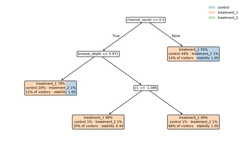
The segmentation came from a policy tree fitted on per-visitor CATEs over every feature column in the observed frame.
Capability detection¶
posterior.has_decomposition()
True
has_decomposition() is True for hurdle posteriors — the fit
produces both a conversion channel and a severity channel, so a
decomposition exists.
posterior.has_credible_segments(threshold=0.90)
True
has_credible_segments(threshold) checks whether any discovered
segment has stability_score >= threshold; the default threshold
is 0.80.
Stability score¶
stability_score is a bootstrap replicability metric, not a posterior
credible-interval width:
Pytyche resamples the per-visitor CATEs with replacement, refits the policy tree on each resample (the posterior is NOT refit — tree refits are seconds), and reports the fraction of refits that recover a matching segment boundary (Jaccard overlap ≥ 0.5 with the original segment’s members).
A score of 1.0 means every bootstrap finds this segment; 0.0 means
it’s a one-off the data happened to support. The default n_bootstrap = 50;
set posterior.fit_policy_tree(n_bootstrap=...) to override. Setting
n_bootstrap=0 skips the bootstrap entirely — segments then carry
stability_score = NaN and a UserWarning is emitted. The bootstrap_seed
kwarg makes bootstrap results deterministic across calls:
tree = posterior.fit_policy_tree(
    max_depth=3,
    min_segment_share=0.10,
    n_bootstrap=50,
    bootstrap_seed=7,
)

for leaf_id, score in tree.stability_scores.items():
    print(f"  leaf {leaf_id}: stability_score={score:.2f}")
  leaf 2: stability_score=1.00
  leaf 4: stability_score=0.44
  leaf 5: stability_score=1.00
  leaf 6: stability_score=1.00
tree.stability_scores is a dict[int, float] keyed by leaf id.
Each segment in tree.segments has a matching id field for lookups:
tree.stability_scores[segment.id] == segment.stability_score.
Per-segment arm best-probabilities¶
for segment in analysis.segments:
    print(f"{segment.rule.description}: {segment.arm_best_probabilities}")
browse_depth <= 0.971455 AND channel in {direct, email, organic, paid}: {'control': 0.2, 'treatment_1': 0.8, 'treatment_2': 0.0}
browse_depth > 0.971455 AND channel in {direct, email, organic, paid} AND z1 <= -1.08555: {'control': 0.0, 'treatment_1': 1.0, 'treatment_2': 0.0}
browse_depth > 0.971455 AND channel in {direct, email, organic, paid} AND z1 > -1.08555: {'control': 0.0, 'treatment_1': 1.0, 'treatment_2': 0.0}
channel == social: {'control': 0.4475, 'treatment_1': 0.5525, 'treatment_2': 0.0}
arm_best_probabilities is a dict keyed by variant name — control
included. Values are the posterior probability that the arm is best in
this segment under the shared best-arm rule (at K=3: the arm with the
largest positive contrast wins; control wins when every contrast is
non-positive). Values sum to 1.0. Use this to:
spot leaves where the engine is confident (one arm dominates) vs ambivalent (two or more arms near-tied)
find drop-treatment candidates (arms with near-zero probability of being best in every segment)
decide per-segment ship vs hold (a segment where the leader has
P > 0.90is shippable; one where it’s0.45against a0.40runner-up is still exploring)
See decision-theoretic inputs for how this composes with the global expected-loss picture.
§3 — Allocation¶
posterior.thompson_allocation(segments, epsilon=0.02) returns the
per-segment treatment mix as a dict[int, dict[str, float]] keyed by
leaf id. Each value is a per-treatment weight dict that sums to 1.0.
allocation = posterior.thompson_allocation(segments=tree.segments)

for segment_id, weights in allocation.items():
    print(f"  segment {segment_id}: {weights}")
  segment 2: {'control': 0.19866666666666666, 'treatment_1': 0.7946666666666666, 'treatment_2': 0.006666666666666667}
  segment 4: {'control': 0.006666666666666667, 'treatment_1': 0.9866666666666667, 'treatment_2': 0.006666666666666667}
  segment 5: {'control': 0.006666666666666667, 'treatment_1': 0.9866666666666667, 'treatment_2': 0.006666666666666667}
  segment 6: {'control': 0.44451666666666667, 'treatment_1': 0.5488166666666666, 'treatment_2': 0.006666666666666667}
The epsilon kwarg is a safety-net floor inside the Thompson
computation (each arm keeps at least ε/K of the leaf’s allocation,
so no arm is starved to zero). It is NOT the dial for how much traffic
stays on control — controls retention is a property of the
experiment’s cell structure, set with min_control_weight and
min_explore_weight on pt.sequential_experiment(...). See
sequential targeting for how
the control, exploration, and optimized cells compose.
The allocation basis is segment_mean — every visitor in a segment
gets the same allocation. Per-visitor allocation is not exposed at
the public surface.
Function-form alternative¶
pt.fit_policy_tree and pt.thompson_allocation are thin function-form
wrappers that delegate to the method forms. The two produce identical results:
# Both forms return the same result:
tree_via_fn = pt.fit_policy_tree(posterior, max_depth=3)
§4 — Decision support¶
posterior.recommendation_summary(treatment, segment) returns the
decision-theoretic snapshot — the inputs you compose into a graduation
rule. segment=None (the default) computes the global snapshot over
all visitors for that treatment’s contrast:
treatment_name = posterior.observed.treatment_names[0]

posterior.recommendation_summary(treatment_name)
RecommendationSummary — treatment_1 vs control
  decision: SHIP
  expected loss — ship now: 0.0000   keep control: 11.2155
  P(lift > 0) = 1.00   P(better) = 1.00   P(harmful) = 0.00
  value of one more round: 0.0000
expected_value_of_one_more_round is the
information-theoretic value of running one more round at the same
per-round n, in outcome units (expected-loss-reduction per visitor).
Near-zero means the experiment has effectively converged and additional
data is unlikely to change the decision.
The standard composition:
Ship when
expected_loss_comparisonis below your tolerance for N consecutive rounds.Continue when
expected_value_of_one_more_roundexceeds the per-visitor cost of another round of latency.Stop when EVOR is at-or-below the round cost AND no contrast has cleared the ship threshold — the experiment has converged on an ambiguous answer.
analysis.recommendation is the same global snapshot for the best
challenger (the treatment with the largest global posterior-mean
contrast). Per-segment snapshots pass a DiscoveredSegment:
posterior.recommendation_summary(treatment_name, segment=analysis.segments[0])
RecommendationSummary — treatment_1 vs control
  decision: CONTINUE
  expected loss — ship now: 0.2542   keep control: 1.6860
  P(lift > 0) = 0.80   P(better) = 0.80   P(harmful) = 0.20
  value of one more round: 0.1083
The library doesn’t have an opinion on your thresholds. See decision-theoretic inputs for the formulas, when to trust them, and an example custom rule.
§5 — Visualization¶
import pytyche.viz as ptviz
pt.viz is lazily imported — matplotlib is only loaded when you
touch pt.viz.*. Each primitive accepts an optional ax= parameter
for subplot composition into an existing figure; when omitted it creates
a fresh figure and returns the Axes.
Forest plot of segment credible intervals:
if analysis.segments:
    ax = ptviz.plot_segment_intervals(analysis.segments)
Policy-tree visualization:
ax_tree = ptviz.plot_policy_tree(tree)
Pass ax=existing_ax to compose either plot into a figure you
manage; the function renders into the provided axes and returns it.
The pt.viz.experiment_evolution_gif(history, ...) animated GIF
primitive (which renders multi-round experiment history) requires the
sequential surface’s Experiment type and arrives with that work.
§6 — Hurdle decomposition¶
For hurdle outcomes — zero-inflated metrics like revenue-per-visitor — the per-visitor effect decomposes into a change in conversion probability (more buyers) and a change in basket size given conversion (larger orders).
if posterior.has_decomposition():
    for comparison in analysis.comparisons:
        print(f"{comparison.treatment} — {comparison.decomposition!r}")
treatment_1 — conversion: +0.0712 [+0.0500, +0.0907]   severity: +34.1756 [+13.2831, +55.3771]
treatment_2 — conversion: -0.0256 [-0.0412, -0.0110]   severity: -24.8586 [-46.4949, -2.0628]
posterior.has_decomposition() returns True for joint hurdle
posteriors and False for continuous or binary posteriors (those have
a single channel; nothing to decompose). Continuous and binary
posteriors expose every other method on this page — only the hurdle
decomposition is hurdle-specific.
§7 — Truth comparison¶
posterior.evaluate_against_truth(tree, truth) is the sim-only
diagnostic. It exists when (and only when) the observed data came
with a planted ground truth — i.e. when you generated the data with
pt.generators.* and have access to bundle.truth. Production
data never has this.
posterior.evaluate_against_truth(tree=tree, truth=truth)
TruthComparison
  cate_rmse: 16.2835   policy_accuracy: 69%
  rpv — policy: 9.9263   uniform: 5.1502   oracle: 11.9873   oracle gap: 2.0610
CATE RMSE — per-visitor error in the recovered conditional treatment effect vs the planted one (pooled across all
n × (K-1)contrast entries at K=3).Policy accuracy — fraction of visitors whose recommended treatment matches the truth-optimal one for their features.
Oracle gap — per-visitor regret of the recommended policy vs an oracle policy that always picks the best treatment.
rpv_policy / rpv_uniform / rpv_oracle — the expected revenue per visitor under the predicted policy, a uniform-allocation baseline, and the oracle policy, respectively. These three together let you quantify how much value the policy tree captures relative to the theoretical maximum.
This is the same comparison the SBC calibration sweep does at scale to fit the R(p) calibration corrections (see BCF posterior calibration at scale). Running it on individual analyses is useful when prototyping a new generator template, validating that the calibration regime matches your domain, or onboarding a new analyst to the library.
Cross-references¶
First adaptive experiment — the narrative tutorial that puts these capabilities in a single end-to-end flow.
Result objects — the type hierarchy and observed-stashing semantics referenced throughout.
Decision-theoretic inputs — the formulas behind §4.
Sequential targeting — why §3’s allocation is structured the way it is.
BCF posterior calibration at scale — the calibration workflow (
apply_calibrationand the R(p) corrections) and why it’s needed. A dedicated hands-on tutorial is planned.Glossary — term definitions.