Running your first adaptive, sequential experiment

You’re a growth PM evaluating three checkout-promotion treatments. You don’t know which works, or for whom — and a standard A/B test won’t tell you: it reports one average lift, hiding exactly the per-customer structure you’d need to target. This tutorial runs an adaptive sequential experiment instead: each round refits a joint hurdle BCF on the cumulative data, refines a decision tree mapping visitor features to recommended treatments, and routes the next round’s traffic through that tree’s segments. One call — pt.sequential_experiment(...) — drives the whole loop.

The experiment is realistically sized: 350,000 visitors across three rounds, end-to-end in about fifteen minutes on a single consumer GPU. That is the point of the library — production-scale Bayesian causal inference on hardware you already have.

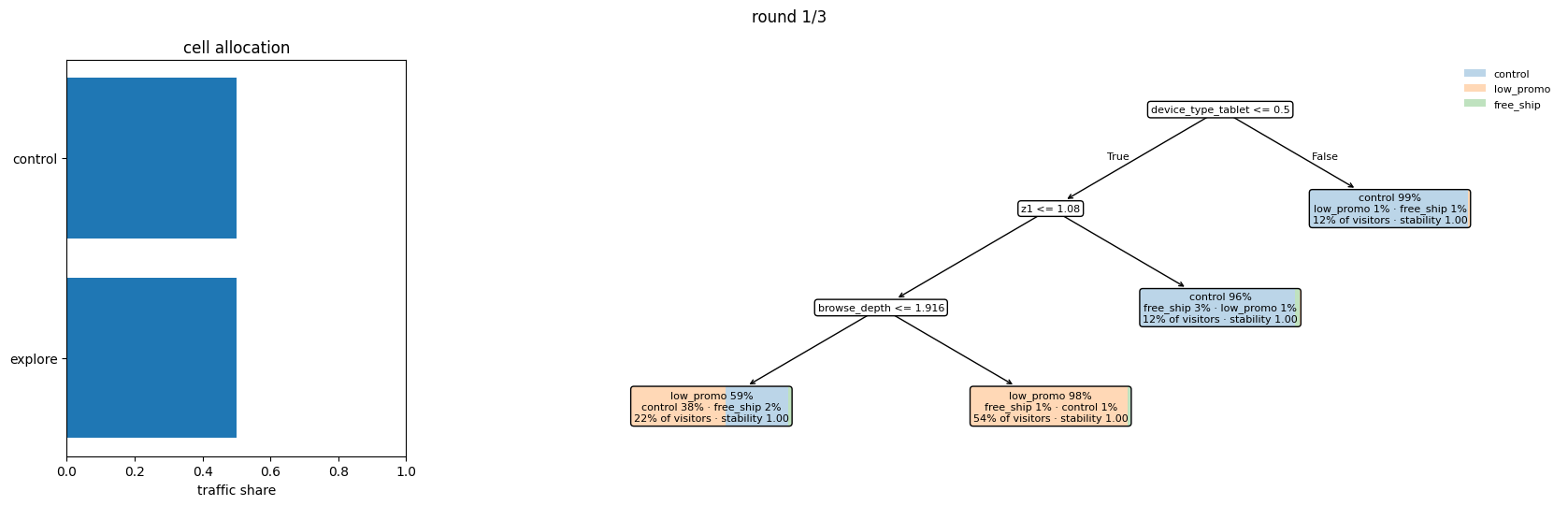
This is the loop you’re about to run — per round, the cell allocation that served traffic and the policy tree it shipped:

Setup

import pytyche as pt

report = pt.check_setup()

pytyche 0.1.0.dev0
bartz   0.9.0
JAX devices: cuda:0
CUDA available: True
calibration artifacts: (none bundled)

The fits in this tutorial expect the CUDA device shown above (on CPU they run, slowly, and warn once). calibration artifacts: (none bundled) is why this tutorial runs uncalibrated.

The scenario

Three candidate checkout-promotion treatments competing for a fixed visitor budget:

• control — no promotion

• low_promo — small storefront promo

• free_ship — free shipping above $50

Three rounds covering 350,000 visitors total, on a doubling-batch schedule (50,000 → 100,000 → 200,000). The data is generated by pytyche’s clustered_realistic template, a four-cluster e-commerce mixture where the best treatment differs by customer cluster.

treatments = ["control", "low_promo", "free_ship"]

generator = pt.simulated_experiment_generator(
    template="clustered_realistic",
    metric="revenue_per_visitor",
    effect_scale=0.1,
    K=3,
    seed=42,
    treatment_names=treatments,
)

schedule = pt.GeometricSchedule(initial=50_000, growth=2.0, n_rounds=3)

pt.simulated_experiment_generator(...) wraps one of pytyche’s data-generating templates as a generator — the callable a sequential experiment pulls each round’s data from. K is the treatment count (control + K−1 active treatments), and treatment_names= maps the template’s arms onto this experiment’s naming. The modest effect_scale plants realistic per-segment effects: large enough to find, small enough that finding them takes data. A real deployment passes its own generator — any callable that pulls a round’s data from your experimentation platform — and everything below stays the same.

Constructing the sequential experiment

pt.sequential_experiment(...) returns a stateful object you iterate round by round. Configuration is fixed at construction. Per-round overrides (custom cells, intervention) happen via the iteration loop.

exp = pt.sequential_experiment(
    generator=generator,
    schedule=schedule,
    treatments=treatments,
    min_control_weight=0.05,
    min_explore_weight=0.05,
    max_segment_depth=3,
    seed=42,
)

Parameters worth understanding before you ship:

• generator is any callable that produces a round’s observed data (and, in sim mode, the corresponding ground truth) when the experiment advances. Real-data runs pass a callable that pulls the round’s data from the experimentation platform.

• min_control_weight=0.05 and min_explore_weight=0.05 are the controls-retention floors. The Control cell never falls below 5% of round traffic. The Explore cell (uniform-random across treatments) also never falls below 5%. Together they guarantee that baseline measurement and every-treatment-observed sampling continue at every round, regardless of how confident the model becomes.

• calibration defaults to None: posteriors are used uncorrected, and every round’s results carry an explicit uncalibrated label. Uncalibrated posteriors are typically overconfident at scale, which also makes allocation concentrate on leaders faster than honest uncertainty would. Passing a calibration artifact instead applies an SBC-fitted coverage correction so posterior intervals stay honest — see calibration at scale for what that corrects and when it matters.

• progress=True (not set here) renders live progress bars over each round’s fit — useful in an interactive notebook while a multi-minute fit runs.

Round 1: cold start

The default round-1 cell structure is a Control cell and an Explore cell at 50/50 share. Half the visitors get the baseline. The other half get a uniform-random treatment, giving the model clean HTE signal to learn from.

r1 = next(exp)

r1

/tmp/ipykernel_298/2702889220.py:1: UncalibratedWarning: Running uncalibrated BCF posteriors (calibration=None); interval coverage may be miscalibrated at scale. Supply an SBC-fitted artifact via sequential_experiment(calibration=...) to correct it.
  r1 = next(exp)

round 0: revenue_per_visitor | 5 segment(s) | SHIP 'low_promo' (P(lift>0)=0.96)

cell	n	RPV (model 80% CI)	lift vs control	policy
control	25,002	2.4060 [2.4514, 2.6565]	—	baseline: always control
explore	24,998	2.5586 [2.5054, 2.6461]	+0.1526 [-0.0556, +0.1293]	uniform over ['control', 'low_promo', 'free_ship']

truth: cate_rmse=0.9884 policy_accuracy=56.7% oracle_gap=0.1089/visitor

next: 3 cell(s), 100,000 visitors

After round 1 the posterior is still finding its footing: there is preliminary signal (the clustered_realistic DGP plants real heterogeneity) but the per-segment picture is not yet settled.

You can inspect the round’s discovered segments directly. Each segment’s gate_estimate is the posterior mean of its segment-level average treatment effect (the GATE), with gate_ci the 80% credible interval (the contracts.py convention, tighter than 95% to bias toward action). stability_score is a bootstrap-replicability score on the segment boundary; segments with stability_score >= 0.80 are considered credible enough to act on.

r1.analysis

AnalysisResult — clustered_realistic-es0.1-seed42-K3 · revenue_per_visitor

comparison	lift (80% CI)	P(lift > 0)
low_promo vs control	+0.2517 [+0.0671, +0.4175]	0.96
free_ship vs control	-0.1338 [-0.3137, +0.0336]	0.15

segment	share	GATE (80% CI)	stability	leader
browse_depth <= 4.66207 AND z0 <= -0.284063 AND z1 <= 1.08033	24%	+0.7324 [+0.4363, +1.0170]	1.00	low_promo P=0.78
browse_depth > 4.66207 AND z0 <= -0.284063 AND z1 <= 1.08033	10%	+1.2363 [+0.6899, +1.8175]	1.00	low_promo P=0.98
browse_depth <= 2.20055 AND z0 > -0.284063 AND z1 <= 1.08033	17%	-0.3321 [-0.6974, -0.0356]	1.00	control P=0.91
browse_depth > 2.20055 AND z0 > -0.284063 AND z1 <= 1.08033	35%	+0.4062 [+0.0482, +0.7227]	1.00	low_promo P=0.93
z1 > 1.08033	14%	-0.7155 [-1.1026, -0.3230]	1.00	control P=0.97

recommendation: SHIP — low_promo

And the recommendation for the next round:

plan = r1.next_recommendation

plan

NextRoundPlan — 100,000 visitors, 3 cell(s)

cell	weight	policy
control	0.05	baseline: always control
explore	0.05	uniform over ['control', 'low_promo', 'free_ship']
optimized	0.90	policy tree routing over 5 segments with per-leaf Thompson allocation

next_recommendation carries the recommended cell structure for the next round. The operator may accept as-is, partially override (for example, add a hypothesis cell alongside the recommended Optimized cell), or fully replace. This tutorial accepts as-is throughout.

ax = pt.viz.plot_cells(plan.cells)

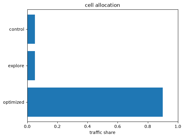
The Optimized cell takes 90% of round-2 traffic; the Control and Explore floors keep their guaranteed 5% shares no matter how confident the model becomes.

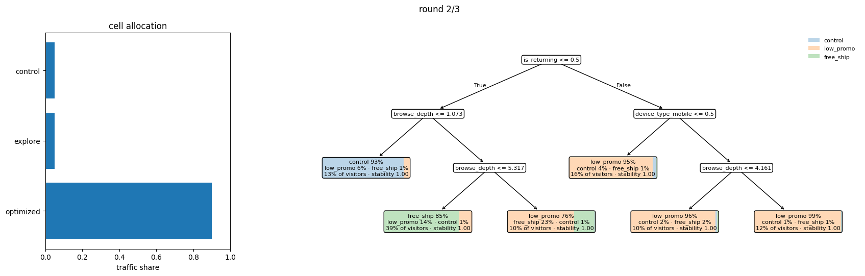
Round 2: narrowing toward responders

r2 = next(exp)

r2

round 1: revenue_per_visitor | 4 segment(s) | SHIP 'low_promo' (P(lift>0)=1.00)

cell	n	RPV (model 80% CI)	lift vs control	policy
control	4,962	2.4665 [2.3952, 2.5358]	—	baseline: always control
explore	4,993	2.6957 [2.4824, 2.6149]	+0.2292 [+0.0059, +0.1399]	uniform over ['control', 'low_promo', 'free_ship']
optimized	90,045	2.6529 [2.6483, 2.7351]	+0.1864 [+0.1476, +0.2967]	policy tree routing over 5 segments with per-leaf Thompson allocation

truth: cate_rmse=0.3491 policy_accuracy=61.8% oracle_gap=0.0982/visitor

next: 3 cell(s), 200,000 visitors

The cumulative posterior now incorporates 150,000 visitors. Round 1’s recommendation introduced an Optimized cell that routes visitors per the policy tree fitted on round 1’s CATEs, and the dashboard’s scoreboard shows whether that targeted routing produced lift over Control — the headline number for the round. The HTE discovery itself is independent of cells: it is a property of the joint posterior over all the data, regardless of how that data was routed.

r2.analysis

AnalysisResult — clustered_realistic-es0.1-seed42-K3 · revenue_per_visitor

comparison	lift (80% CI)	P(lift > 0)
low_promo vs control	+0.2680 [+0.1577, +0.3798]	1.00
free_ship vs control	-0.0589 [-0.1926, +0.0663]	0.29

segment	share	GATE (80% CI)	stability	leader
browse_depth <= 1.13612	17%	-0.1177 [-0.3181, +0.0653]	1.00	control P=0.77
browse_depth > 1.13612 AND channel in {direct, email, organic, paid} AND z1 <= 1.08344	63%	+0.4005 [+0.2860, +0.5126]	1.00	low_promo P=0.99
browse_depth > 1.13612 AND channel in {direct, email, organic, paid} AND z1 > 1.08344	10%	+0.2535 [-0.2796, +0.4920]	1.00	low_promo P=0.78
browse_depth > 1.13612 AND channel == social	10%	+0.0393 [-0.3715, +0.5043]	0.94	low_promo P=0.43

recommendation: SHIP — low_promo

ax = pt.viz.plot_segment_intervals(r2.analysis.segments)

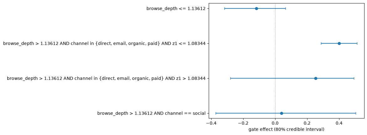
Expect narrower credible intervals than round 1, and the per-segment leaders to firm up. arm_best_probabilities (rendered per segment above) is the per-segment posterior probability that each arm is best — a leaf where the leader sits above 0.90 is one the engine is confident in, while a leader at 0.45 against a 0.40 runner-up is still exploring. The experiment exposes predicate accessors for the common questions:

{
    "credible segments yet": exp.has_credible_segments(),
    "graduation candidate yet": exp.has_graduation_candidate(),
}

{'credible segments yet': True, 'graduation candidate yet': True}

has_credible_segments() answers “is any segment credible”; has_graduation_candidate() answers “is any (treatment, segment) pair ready to ship.” With effects this clear, the first graduation candidate often appears as early as round 2 — the floors keep the experiment honest either way. The actual candidate list comes from exp.graduation_candidates(...) (round 3, below).

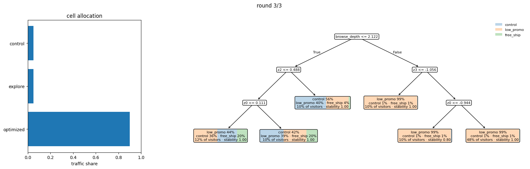
Round 3: mature segmentation

r3 = next(exp)

r3

round 2: revenue_per_visitor | 5 segment(s) | SHIP 'low_promo' (P(lift>0)=1.00)

cell	n	RPV (model 80% CI)	lift vs control	policy
control	10,043	2.2150 [2.4135, 2.5027]	—	baseline: always control
explore	10,050	2.5818 [2.4624, 2.5310]	+0.3668 [+0.0029, +0.0873]	uniform over ['control', 'low_promo', 'free_ship']
optimized	179,907	2.7793 [2.7350, 2.7986]	+0.5643 [+0.2657, +0.3563]	policy tree routing over 4 segments with per-leaf Thompson allocation

truth: cate_rmse=0.2989 policy_accuracy=67.2% oracle_gap=0.0677/visitor

next: 3 cell(s), no next round (schedule exhausted)

After three rounds and 350,000 cumulative visitors, the policy tree’s segmentation has matured. The default graduation rule (ExpectedLossRule, evaluated over each round’s recommendation_summary decision evidence) fires for a (treatment, segment) pair when all three conditions hold across consecutive rounds: expected loss below tolerance, probability of outperforming control above 0.95, and probability of meaningful improvement above 0.80.

candidates = exp.graduation_candidates(sustained_rounds=2)

candidates[0]

GraduationCandidate — 'low_promo' @ browse_depth > 1.07424 AND channel in {direct, email, social}, sustained 3 round(s)
  expected loss if shipped: 0.0000/visitor   P(lift > 0) = 1.00
  value of one more round: 0.0000/visitor

A run at this scale typically graduates one to three (treatment, segment) pairs by round 3 — the cell shows the first; candidates holds them all. Each candidate is structured data. The operator (or an automated workflow) decides whether to promote one to broader rollout. The library does not auto-ship.

The candidate’s latest_recommendation carries the full decision evidence, including expected_value_of_one_more_round: the expected per-visitor reduction in regret from running one more round at the same per-round n. A candidate where this value is near zero is one the experiment has effectively converged on — additional data is unlikely to change the decision. A non-zero value means you’re still data-limited; ship only if the time-cost of another round exceeds the expected gain. See decision-theoretic inputs for the formula and the compose-into-your-policy framing.

What to do with the result

print(exp.summary)

3 round(s) completed; confidence is high. Latest round 2: revenue_per_visitor | 5 segment(s) | SHIP 'low_promo' (P(lift>0)=1.00)

We have strong, sustained evidence: at least one discovered segment is stable across bootstrap refits, and a treatment has met the graduation thresholds in consecutive rounds. This round's summary decision is SHIP — the leading treatment clears the decision thresholds on the current evidence.

Next round: no further rounds (the schedule is exhausted), split control 5%, explore 5%, optimized 90%. The optimized cell routes through a policy tree over 5 discovered segment(s) with per-segment Thompson allocation.

Graduation candidates (surfaced for the operator — nothing is auto-graduated): low_promo in segment 4 (browse_depth > 1.07424 AND channel in {direct, email, social}); low_promo in segment 5 (browse_depth > 1.07424 AND channel == paid); low_promo in segment 7 (browse_depth > 1.07424 AND channel == organic AND z4 <= 0.468919); low_promo in segment 8 (browse_depth > 1.07424 AND channel == organic AND z4 > 0.468919).

Graduation candidates: low_promo in segment 4; low_promo in segment 5; low_promo in segment 7; low_promo in segment 8.

exp.confidence

'high'

exp.summary is a multi-paragraph prose summary of the latest round in the context of the experiment’s history. exp.confidence is a one-word label ("high", "medium", or "low") derived from the credible-segment count and graduation candidate state, useful for at-a-glance status in a notebook or dashboard.

For platform handoff, exp.next_recommendation is the next-round cell structure your experimentation platform would consume. The structured Python dataclass is the canonical output. Platform integrations convert it to whatever shape the target configuration store expects.

Sim-mode truth comparison

Because this tutorial runs against a generator, each round carries a truth comparison: the planted ground truth against the round’s estimate. Real-data runs (where the generator returns truth=None) skip these.

r3.truth_comparison

TruthComparison
  cate_rmse: 0.2989   policy_accuracy: 67%
  rpv — policy: 2.7891   uniform: 2.5434   oracle: 2.8568   oracle gap: 0.0677

Policy accuracy is the fraction of visitors for whom the recommended treatment matches the truth-optimal treatment. Oracle gap is the RPV regret of the recommended policy versus the oracle policy.

Round-by-round history

The full per-round snapshots are attached to the experiment.

for past in exp.history:
    print(past.summary_one_line())

round 0: revenue_per_visitor | 5 segment(s) | SHIP 'low_promo' (P(lift>0)=0.96)
round 1: revenue_per_visitor | 4 segment(s) | SHIP 'low_promo' (P(lift>0)=1.00)
round 2: revenue_per_visitor | 5 segment(s) | SHIP 'low_promo' (P(lift>0)=1.00)

Each entry carries the round’s posterior, comparisons, summary recommendation, discovered segments, cells shipped, per-cell observations, and recommendation for the next round.

The same evolution visually, one panel per round:

What’s next

This tutorial walked the simplest workflow: accept the recommended tree each round. From here:

• The injecting your own treatment hypotheses tutorial shows how to add your own cells alongside the recommended cell structure when you have a theory you want to test in parallel.

• Advanced experimental design covers the statistical and budget knobs — graduation thresholds, control/explore floors, segmentation depth, schedule shape — and how to choose them for your domain.

• The calibration at scale concept doc explains what a calibration artifact corrects and why this tutorial’s uncalibrated run (the calibration=None default) is the right starting point but not the production recommendation.

• Statistical honesty explains why discovered-segment claims need the stability scores and credible intervals you saw above — and what goes wrong with post-hoc dashboard mining.

• The glossary defines every term used here.