Experiment structure: cells and allocation

An adaptive experiment has three jobs that pull in different directions: measure honestly (you need a live control reference, forever), learn what works for whom (every arm needs data in every kind of visitor, or you can’t tell), and earn (once you know what works, traffic spent elsewhere is money left on the table). Pytyche’s answer is structural: each round’s traffic is split into cells, and each cell does exactly one of those jobs.

This page explains the canonical cell structure and the allocation rule inside it — with pictures. The full design rationale lives in sequential targeting; the hands-on walkthrough is the first adaptive experiment tutorial.

The canonical three cells

Every round the recommendation engine proposes the same three-cell shape (weights are the operator’s dials, min_control_weight / min_explore_weight on pt.sequential_experiment(...); defaults shown):

from types import SimpleNamespace

import pytyche as pt

# plot_cells reads `id` and `weight` — in real use you pass the
# engine's own cells (`plan.cells`), as the adaptive tutorial does.
layout = [
    SimpleNamespace(id="control", weight=0.05),
    SimpleNamespace(id="explore", weight=0.05),
    SimpleNamespace(id="optimized", weight=0.90),
]
pt.viz.plot_cells(layout);

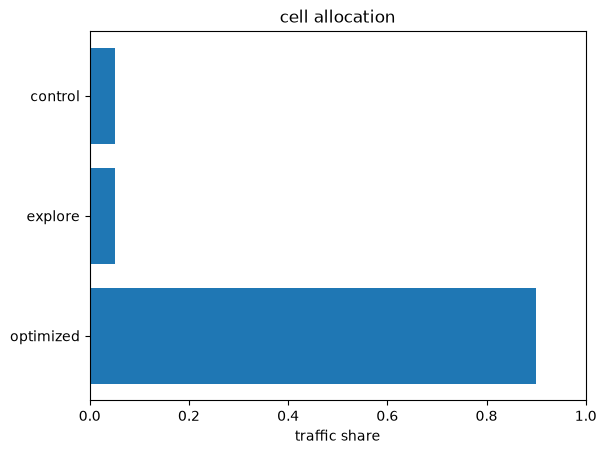
• Control — everyone gets the baseline. This is the permanent measurement reference: however confident the model gets, lift is always “compared to a live control,” never “compared to what we remember.” It is also never droppable.

• Explore — uniform random over all active arms, ignoring the model entirely. This is the floor that keeps the experiment identified: every arm keeps receiving data in every segment, so the model can always re-estimate any arm anywhere — including noticing that an arm it wrote off has started working (population drift, product changes).

• Optimized — the remaining ~90%, routed by the current policy: a shallow decision tree assigns each visitor to a discovered segment, and the segment’s allocation decides which arm they get.

The first two cells are deliberately dumb. All of the model’s intelligence is concentrated in the third — which is what the rest of this page is about.

Inside the Optimized cell: Thompson allocation

Within a segment, each arm’s traffic share is the posterior probability that it is the segment’s best arm. That single sentence is the whole allocation rule (Thompson sampling, at segment granularity). Mechanically: each posterior draw casts a vote for the arm it shows winning in that segment — control wins a draw exactly when no treatment shows a positive lift — and an arm’s share is its win frequency over draws.

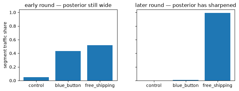
The consequence is the behavior you actually want from an adaptive experiment, with no thresholds to tune. Early on, when the posterior is still wide, contending arms split the segment’s traffic — so the next round gathers evidence exactly where the decision is open. As evidence accumulates and the posterior sharpens, traffic concentrates on the winner:

import matplotlib.pyplot as plt
import numpy as np

rng = np.random.default_rng(0)
arms = ["control", "blue_button", "free_shipping"]


def thompson_weights(mean, sd, n_draws=4000):
    """Win frequency per arm over posterior draws of the two lifts."""
    draws = rng.normal(mean, sd, size=(n_draws, 2))  # lifts vs control
    best = np.where(draws.max(axis=1) <= 0, 0, draws.argmax(axis=1) + 1)
    return np.bincount(best, minlength=len(arms)) / n_draws


early = thompson_weights(mean=[0.04, 0.05], sd=0.06)  # round 1: wide
late = thompson_weights(mean=[0.01, 0.06], sd=0.015)  # round 4: sharp

fig, axes = plt.subplots(1, 2, figsize=(9, 3), sharey=True)
for ax, w, title in [
    (axes[0], early, "early round — posterior still wide"),
    (axes[1], late, "later round — posterior has sharpened"),
]:
    ax.bar(arms, w)
    ax.set_title(title)
axes[0].set_ylabel("segment traffic share");

Two properties worth noticing:

• Exploration costs almost nothing. Thompson only splits traffic between arms that are near-tied — and when arms are near-tied, the value difference between them is, by definition, small. Where one arm clearly dominates, it gets nearly everything.

• Control is a first-class arm. A segment where every treatment looks harmful allocates its traffic back to control automatically — “do nothing here” is a discoverable answer, not a failure mode.

Each segment gets its own mixture, so one round can simultaneously be exploiting a resolved segment and still actively comparing arms in a contested one. The pt.viz.plot_policy_tree rendering shows this per-leaf: each leaf is labeled with its leading arm and its current allocation.

Watching a whole experiment

Put the pieces together over rounds and the structure becomes visible: the cell layout stays fixed while, inside the Optimized cell, the policy tree’s segments and their allocations evolve as the posterior learns. pt.viz.experiment_evolution_gif(exp.history, path) renders this directly from an experiment’s history — this is the canonical adaptive tutorial’s run:

Read it round by round: allocations start spread within each segment, then concentrate as the posterior sharpens; segments themselves can split or merge as the refit tree finds sharper structure; and the Control and Explore floors persist untouched throughout — the measurement and identification guarantees don’t decay as the experiment gets confident.

Why this shape

The structure separates two duties that are tempting to conflate:

• The floors are flat on purpose. Control and Explore provide guarantees — a live reference, identification everywhere, drift detectability — and guarantees shouldn’t depend on what the model currently believes. They are sized by operator policy, not by posterior state.

• The adaptivity is concentrated and self-pricing. All model-driven traffic shifting happens inside the Optimized cell, through a rule whose exploration spend is automatically proportional to how unresolved each decision is — and whose cost is lowest exactly where its spread is largest.

Assignment probabilities are recorded exactly for every visitor in every cell, so the accumulated data stays analyzable across rounds no matter how the allocation evolved.

These guarantees are bought with flat spend — the floors cost the same whether or not the posterior still needs them. The structures below price that trade differently.

Other experiment structures

Forward-looking design intent — not shipped behavior

This section describes design direction for upcoming releases; today’s engine ships the three-cell structure above.

The three-cell Thompson structure is one point on a spectrum of equally valid designs, and it is the hybrid point: structural floors around an adaptive core. The two pure endpoints are:

• Continuous batched Thompson — one cell. Since Thompson already spreads traffic where the posterior is uncertain and already treats control as a first-class arm, the floors can be folded into the allocation itself: a single cell whose policy is the per-segment Thompson mixture, with the round-1 allocation informed by prior beliefs (a flat prior gives a uniform first round — the Explore cell’s job, done by the same rule that handles every later round) and minimum shares expressed as floor parameters rather than as separate cells. Maximally adaptive; nothing is spent on flat floors the posterior has already resolved past.

• Deterministic policies as cells. Each segment gets 100% of its optimized traffic from its current best arm, and alternatives are tested via challenger cells carrying alternate segment-to-arm mappings. A set of deterministic cells with weights induces exactly a per-segment traffic mixture, so nothing statistical is forfeited — what changes is legibility: each cell is a complete, nameable policy you could ship, and the cell-level scoreboard compares deployable policies head-to-head.

All three structures rest on the same statistical machinery — recorded assignment probabilities, accumulated-data refits, per-segment posterior contrasts — and differ in where they put exploration and how auditable the moving parts are. The intended direction is for the library to support these structures as first-class options — including sizing challenger cells by the value of resolving the remaining uncertainty (the expected_value_of_one_more_round machinery from the decision-theoretic inputs) rather than by uncertainty alone. The building blocks are already public: Cell, TreePolicy, and arbitrary allocation maps.

Related pages

• Sequential targeting — the full design rationale for the loop this structure serves.

• Decision-theoretic inputs — the quantities that decide when a treatment graduates out of the loop.

• First adaptive experiment — the end-to-end tutorial this page’s GIF comes from.

• Working with the posterior — thompson_allocation and fit_policy_tree in isolation.